Advanced Tutorials¶

Moving beyond standard CLI usage, this guide walks you through more advanced, hands-on examples. You will learn how to:

Execute queries directly through Python objects
Construct leak-free train/validation/test splits for your curated datasets
Perform post-export dataset audits
Curate and refine chemistry data

These examples build upon the CLI command references, configuration reference, and query examples.

Note

These examples illustrate the workflow — adapt the thresholds and methods to your own data and scientific requirements.

Prerequisite: This guide assumes you have already created a processed query database (Parquet files) during the process step.

Shared Setup¶

All examples in this guide use the QueryDatabaseHandler class to interact with your query database — see the examples below for how to construct and use it. You can initialize it with the default reader for standard paths, or inject a custom reading function for specialized I/O requirements.

Option A: Default Setup (Standard Local/S3 Path)¶

Use this approach for standard local directories or cloud storage URIs where default reading rules apply:

from chemreporter.query_database_tools.query_database import QueryDatabaseHandler

db_path = "path/to/query_database"  # local path or "s3://my-bucket/db"
db_query = QueryDatabaseHandler(db_path)

Option B: Custom Reader Function¶

If your project requires specific storage options or custom loading logic, you can pass your own reader function:

import polars as pl
from cloudpathlib import AnyPath

from chemreporter.query_database_tools.query_database import QueryDatabaseHandler


def custom_read_parquet(
    file_path: AnyPath,
) -> pl.LazyFrame:
    """Custom parquet reader applying project-specific storage options."""
    return pl.scan_parquet(str(file_path))


db_path = AnyPath("path/to/query_database")  # local path or s3:// URI
db_query = QueryDatabaseHandler(db_path, read_func=custom_read_parquet)

Querying and Filtering Data¶

Begin by filtering entries based on specific molecular properties, using the db_query object created above. The API accepts SQL-like syntax, allowing you to filter across any schema field seamlessly.

query = "net_force_norm < 1.0e-3 AND "
query += "max_force_norm < 15 AND "
query += "is_molecular_structure_valid"

keys = db_query.query_to_keys(query)

This is what you would see, for instance, if your query database has OMOL25 processed into it:

🔍 Query: net_force_norm < 1.0e-3 AND max_force_norm < 15 AND is_molecular_structure_valid
✅ Found 103,699,333 molecules matching the criteria

To extract a subsample of the query results, simply pass the sampling keyword arguments:

keys_sampled = db_query.query_to_keys(
    query, sampling_method="random", n_samples=1000
)

Matching keys feed directly into three built-in analysis actions, each operating on the same db_query object and the same array of entry keys: make_histograms plots a histogram for one or more columns, make_statistics writes summary statistics (count, mean, min, max, …) to a CSV file, and extract_smiles extracts the SMILES strings of the matched entries into a .npy file. All three are importable from chemreporter.query_database_tools.actions_tools. The example below plots a histogram of max_force_norm:

from pathlib import Path

from chemreporter.query_database_tools.actions_tools import make_histograms

make_histograms(
    db_handler=db_query,
    entry_keys=keys_sampled,
    output_path=Path("/path/to/output_dir"),
    column_names=["max_force_norm"],
)

Save these keys to a file (e.g., filtered_keys.npy), and you have exactly what the HDF5 export step requires.

To explore available query fields, you can inspect FULL_SCHEMA. It provides comprehensive documentation, including field names and descriptions, eliminating any guesswork:

from chemreporter.query_database_tools.table_schemas import FULL_SCHEMA

for field in FULL_SCHEMA:
    print(f"{field.name}: {field.description}")

If the built-in actions aren’t enough, db_query.get_dataframe(indices=keys, columns=[...]) gives you the raw Polars DataFrame for the matched keys, so you can filter, join, or transform it however your analysis requires. The next sections rely on this, too.

Constructing Leak-Free Data Splits¶

To avoid data leakage, split by molecular identity, not by row: if the same molecule (identified by its canonical smiles) ends up in both your training and test sets — even as a different conformation or with a different label — your test metrics stop measuring generalization to unseen chemistry. Splitting on unique smiles values, rather than randomly across all rows, keeps every occurrence of a given molecule on the same side of the split.

Reactive datasets add another axis of leakage on top of this: structures along the same reaction pathway (e.g. reactant, transition state, product) share the same underlying reaction, so splitting them across training and test still leaks information about that reaction. For these datasets, partition by unique reaction_id instead of smiles — the example below does exactly that for the RGD subset of OMOL25, and generalizes directly to a plain molecule split if you swap reaction_id for smiles throughout.

One effective, leakage-free approach is to fetch the reaction_id for the entry keys returned by your query (see Querying and Filtering Data), collect the unique reaction IDs, shuffle them, and slice the shuffled list by your desired fractions:

df = db_query.get_dataframe(indices=keys, columns=["entry_key", "reaction_id"])
unique_reaction_ids = df.select("reaction_id").unique().collect()

# Shuffle the reaction_ids to ensure randomization
unique_reaction_ids = unique_reaction_ids.sample(fraction=1.0, shuffle=True, seed=42)

n = unique_reaction_ids.height

# Allocate 90% of the unique reactions to the training set
n_train = int(0.90 * n)
training_reaction_ids = unique_reaction_ids.slice(0, n_train)
validation_reaction_ids = unique_reaction_ids.slice(n_train)

train_keys = (
    df.join(training_reaction_ids.lazy(), on="reaction_id", how="inner")
    .select("entry_key")
    .collect()
    .sample(n=20000, seed=42)
    .get_column("entry_key")
    .to_numpy()
)

validation_keys = (
    df.join(validation_reaction_ids.lazy(), on="reaction_id", how="inner")
    .select("entry_key")
    .collect()
    .sample(n=2000, seed=42)
    .get_column("entry_key")
    .to_numpy()
)

Running this over the RGD subset of OMOL25 (3,359,478 entries spanning 140,672 unique reaction IDs) yields clean, isolated datasets:

There are 66115 training reaction ids

We have 20000 samples in the training split covering 16971 unique reaction ids
We have 2000 samples in the training split covering 1452 unique reaction ids

You can then save each split’s train_keys / validation_keys array of entry keys as a NumPy file, which is exactly what chemreporter export needs to finalize the datasets.

Restricting Queries with Allowlists¶

When your target molecules are predetermined — such as a held-out training set, or a previously defined split like training_reaction_ids above — you can apply an allowlist directly within the query. The restrict_to parameter performs an efficient semi-join, eliminating the need for post-query filtering:

keys = db_query.query_to_keys(
    query,
    n_samples=100000,
    restrict_to={"columns": ["reaction_id"], "values": training_reaction_ids},
)

The columns argument can accept multiple fields. In such cases, a row must match on all specified fields, allowing you to enforce composite identities like ["reaction_id", "reaction_pathway_id"].

If you are using a YAML config file instead of the Python API, the allowlist is provided as path_to_values, pointing to a file instead of a DataFrame: a .npy file for a single column’s values, or a .npz file containing one named array per column:

restrict_to:
  columns: reaction_id
  path_to_values: path/to/allowlist.npy

Dataset Analysis¶

Exported key files don’t store the metadata themselves — they are exact pointers back into your query database. You can load a saved key array back in at any time and use db_query.get_dataframe (introduced in Querying and Filtering Data) to pull any schema field into a DataFrame for further analysis, which is particularly useful for comparing the property distributions of different sampling strategies, for example a random baseline against the diversity-based sampling strategies from Sampling:

import numpy as np

baseline_keys = np.load("path/to/non_greedy_keys.npy", allow_pickle=True)
sampled_keys_a = np.load("path/to/sampled_selection_a.npy", allow_pickle=True)
sampled_keys_b = np.load("path/to/sampled_selection_b.npy", allow_pickle=True)

columns = ["num_atoms", "logp", "dipole_moment_magnitude"]
df_baseline = db_query.get_dataframe(indices=baseline_keys, columns=columns).collect()
df_sampled_a = db_query.get_dataframe(indices=sampled_keys_a, columns=columns).collect()
df_sampled_b = db_query.get_dataframe(indices=sampled_keys_b, columns=columns).collect()

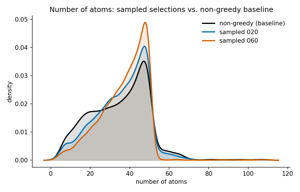
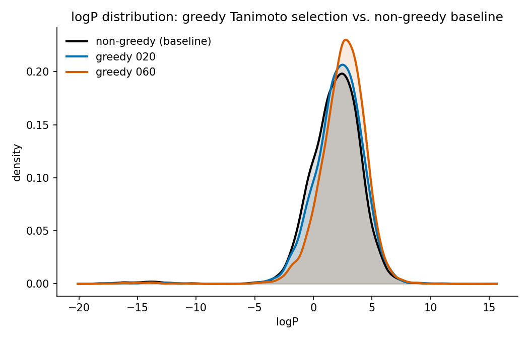
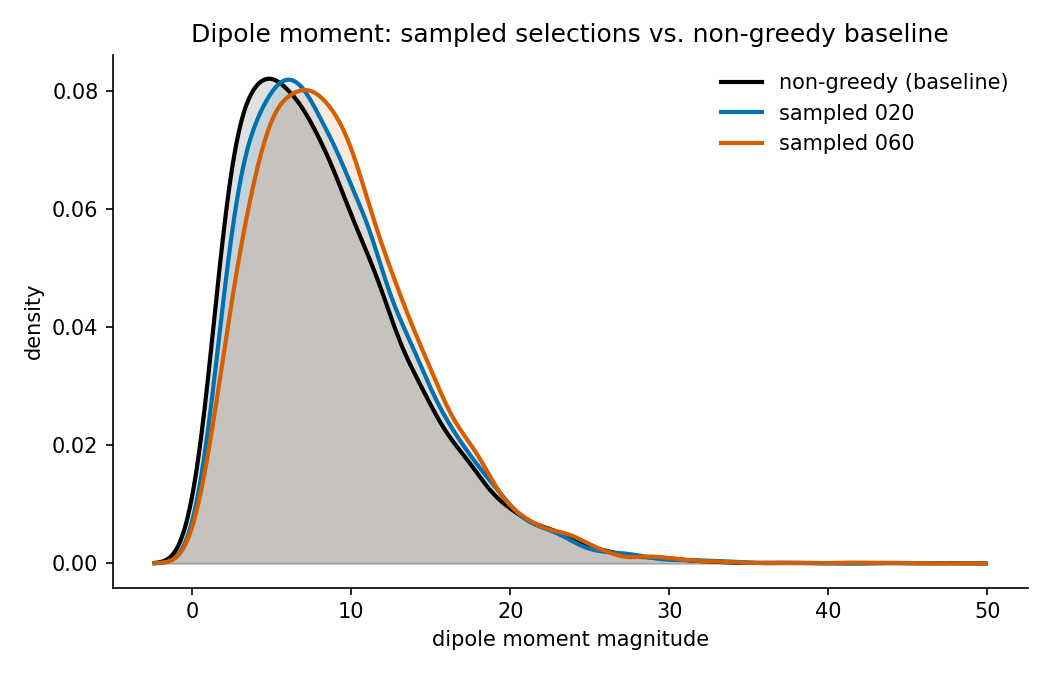
The plots below compare the resulting property distributions of the two sampled selections against the random (non_greedy) baseline:

Number of atoms: sampled selections vs. non-greedy baseline

logP distribution: sampled selections vs. non-greedy baseline

Dipole moment: sampled selections vs. non-greedy baseline

Note

If the original key file is lost, you can extract the keys directly from the exported HDF5 file itself — its top-level groups are the entry keys.

Curating a Dataset: Reactive Chemistry (Transition States)¶

Using reaction-pathway data (such as the rgd subset of OMOL25), you can programmatically derive transition-state labels from energy profiles, filter out unphysical pathways, and construct perfectly balanced splits.

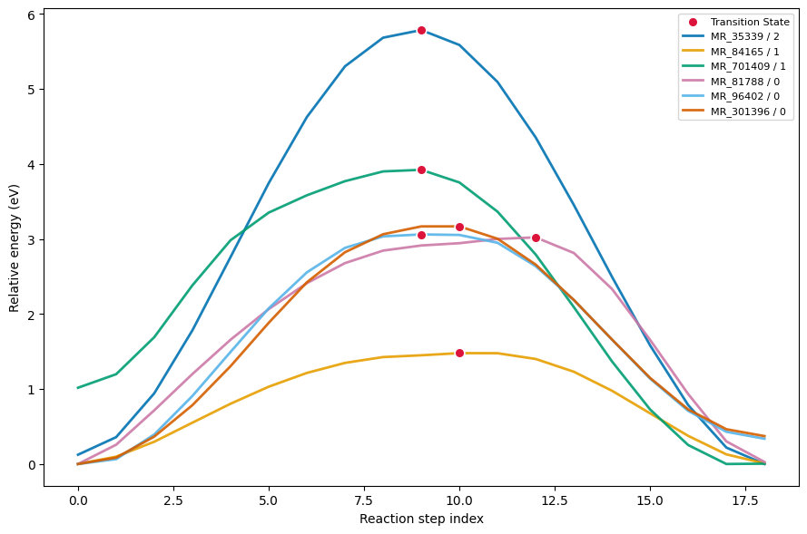
We define the transition state (TS) of a reaction pathway as the point of maximum energy along that pathway, then discard profiles whose maximum falls on the reactant or product endpoint, since those don’t represent a real energy barrier. In the example below, df is a Polars DataFrame for the rgd subset — for example fetched via db_query.get_dataframe(indices=keys, columns=[...]) with at least reaction_id, reaction_pathway_id, reaction_step_idx, and energy — and filter_expr is your own row filter (e.g., excluding already-known-bad geometries) applied before the TS search; use pl.lit(True) if you don’t need one:

import polars as pl

# Label each row True when its energy equals the max energy of its own
# pathway (grouped by reaction_id + reaction_pathway_id), among the rows
# that satisfy filter_expr. Every other row is labeled False.
df_with_ts = df.with_columns(
    pl.when(filter_expr)
    .then(
        (
            pl.col("energy")
            == pl.col("energy").max().over(["reaction_id", "reaction_pathway_id"])
        ).cast(pl.Boolean)
    )
    .otherwise(False)
    .alias("is_ts")
)

# Find the pathways whose transition state falls on step 0 (the reactant)
# or step 18 (the product)—indicating an endpoint, not a real energy barrier.
df_reactant_or_product_is_ts = (
    df_with_ts.filter(
        (pl.col("is_ts"))
        & ((pl.col("reaction_step_idx") == 0) | (pl.col("reaction_step_idx") == 18))
    )
    .select(["reaction_id", "reaction_pathway_id"])
    .unique()
)

# Remove those unphysical pathways from the dataset via an anti-join.
filtered_df_with_ts = df_with_ts.join(
    df_reactant_or_product_is_ts,
    on=["reaction_id", "reaction_pathway_id"],
    how="anti",
)

Percentage of pathway_ids with TS at step 0 or 18: 1.13 %
Total number of profiles removed (both filtering steps): 27.09 %

After additionally filtering out multi-maximum profiles (not shown), every remaining curve is single-peaked with exactly one valid transition state:

Energy profiles after curation

Finally, you can sample the curated data to achieve target class proportions using a weighted sampler. filtered_df_with_weights below is filtered_df_with_ts after that additional filtering, with a weight column you compute so that a random draw matches target_ratios; the already-populated is_reactant / is_product boolean columns identify the other two classes, and sample_size is the total number of rows you want in the final sample:

target_ratios = {"is_ts": 0.2, "is_product": 0.4, "is_reactant": 0.4}
sample = filtered_df_with_weights.sample(sample_size, weights="weight")

is_ts ratio: 0.20
is_product ratio: 0.40
is_reactant ratio: 0.39
Unique reactions: 18514

Retrieving Original Source Data¶

Because entry keys are entirely self-describing — encoding the dataset, split, file, and row index — you never need a separate lookup table to trace a record back to its origin:

shape: (5, 4)
┌───────────────────┬──────────────┬────────┬───────────────────────────────┐
│ reaction_step_idx ┆ energy       ┆ subset ┆ entry_key                     │
╞═══════════════════╪══════════════╪════════╪═══════════════════════════════╡
│ 14                ┆ -9934.600177 ┆ rgd    ┆ omol25_train_data0020_916944  │
│ 2                 ┆ -10306.79811 ┆ rgd    ┆ omol25_train_data0039_1264980 │
└───────────────────┴──────────────┴────────┴───────────────────────────────┘

If a specific field was omitted from the query database during processing, you can retrieve it directly from the original source dataset. This needs db_path (the same query database path from Shared Setup above) and a ChemReporterIO instance to handle the download — here we look up the source field for the first key returned by an earlier query:

from chemreporter.cli.io_utils import ChemReporterIO
from chemreporter.source_database_tools.fetch import fetch_source_database_readers
from chemreporter.source_database_tools.utils import (
    retrieve_source_database_data_from_keys,
)

io = ChemReporterIO()
source_db_readers = fetch_source_database_readers(
    db_path, download_function=io.download_file
)
retrieved_data = retrieve_source_database_data_from_keys(
    source_db_readers, [keys[0]], data_field="source"
)

Warning

This operation downloads the original source database and can be slow. It is highly recommended to retrieve only a few keys at a time, or to run this process in an environment where the source data is already stored locally.

For complete command-line usage, refer to the CLI Reference. For a detailed breakdown of field definitions available for queries, see the Database Schema.